Nowcasting on Structured data
Rafael Lopes & Leonardo Bastos
Source:vignettes/articles/1_structured_data.Rmd
1_structured_data.RmdTL;DR
This is a more length article explaining the workings and the choices behind the nowcasting model and its advantages and limitations.
As Before…
As in the Get Started we start by loading the package and its lazy data, by:
Non-structured data
The Get Started example is done on non-structured data, here we give a more detailed description of this type of data and how it can change the nowcasting.
When we call the nowcasting_inla() function, it has by
default the parameterization to take the data and estimate with a
non-structured data form. The estimate fits a negative binomial
distribution,
,
to the cases count at time
with delay
,
is the dispersion parameter. The rate
is then parametric in a log-linear format by a constant term added by
structured delay random effects and structured time random effects. This
is the whole premise of nowcasting, we model the case counts at time
given the case count at that time and past values as well as given the
delay distribution of that count.
Hence, the model is given by the following:
$$\begin{equation} Y_{t,d} \sim NegBinom(\lambda_{t,d}, \phi) \\ \log(\lambda_{t,d}) = \alpha + \beta_t + \gamma_d \\ \beta_t := u_t - u_{(t-1)} - u_{(t-2)} \sim N(0,\tau_{\beta}); \gamma_d := u_d - u_{(d-1)} \sim N(0, \tau_{\gamma})\\ t=1,2,\ldots,T \\ d=1,2,\ldots,D \\ \end{equation}$$
Where the intercept
follows a Gaussian distribution with a very large variance,
follows a second order random walk with precision
,
while
a first-order random walk with precision
.
The model is then completed by INLA default prior distributions for
,
,
and
.
See nbinomial,
rw1
and rw2
INLA help pages.
The call of the function is straightforward, it simply needs a data
set as input, here the LazyData loaded in the namespace of
the package. The function has 3 mandatory parameters,
dataset to parse the data set to be nowcasted,
date_onset for parsing the column name which is the date of
onset of symptoms and date_report which parses the column
name for the date of report of the cases. Here this columns are
“DT_SIN_PRI” and “DT_DIGITA”, respectively. Need for two dates is due to
we are modeling the delay as part of the nowcasting estimation, usually
nowcasting models assuming a delay distribution and apply it to the
cases observed.
nowcasting_bh_no_age <- nowcasting_inla(dataset = sragBH,
                                        date_onset = DT_SIN_PRI,
                                        date_report = DT_DIGITA)
head(nowcasting_bh_no_age$total)
#> # A tibble: 6 × 7
#>    Time dt_event   Median    LI    LS   LIb   LSb
#>   <int> <date>      <dbl> <dbl> <dbl> <dbl> <dbl>
#> 1    17 2021-12-13    444   442  448    443   445
#> 2    18 2021-12-20    632   626  640    629   634
#> 3    19 2021-12-27    736   728  750.   732   740
#> 4    20 2022-01-03    759   746  778    754   765
#> 5    21 2022-01-10    879   862  905    872   887
#> 6    22 2022-01-17    785   764  815    777   795
The above calling will return only the nowcasting estimate and its
Confidence Interval (CI) for two different credibility levels,
LIb and LSb are the max and min CI,
respectively, with credibility of 50% and LI and
LS are the max and min CI, respectively, with credibility
of 95%.
The nowcasting_inla has the option to return the curve
on which the window of action of the model was set, if the
data.by.week parameter is flagged as TRUE it
returns on the second element of the output list, the summarized data by
week.
nowcasting_bh_no_age <- nowcasting_inla(dataset = sragBH,
                                        date_onset = DT_SIN_PRI,
                                        date_report = DT_DIGITA,
                                        data.by.week = T)
head(nowcasting_bh_no_age$data)
#> # A tibble: 6 × 4
#>   dt_event   delay     Y  Time
#>   <date>     <dbl> <dbl> <int>
#> 1 2021-08-23     0     8     1
#> 2 2021-08-23     1    70     1
#> 3 2021-08-23     2    92     1
#> 4 2021-08-23     3    68     1
#> 5 2021-08-23     4    32     1
#> 6 2021-08-23     5    32     1
This element is the counts of cases by each delay days. It is known as the delay triangle, if we table the delay amount against the date of onset of first symptoms, we can see the pattern of the delay for the cases.
library(dplyr)

data_triangle <- nowcasting_bh_no_age$data |>
  filter(delay < 30) |>
  arrange(delay) |>
  select(-Time)

data_triangle |>
  filter(dt_event >= (max(dt_event) - 84),
         delay <= 10) |>
  tidyr::spread(key = delay, value = Y)
#> # A tibble: 13 × 12
#>    dt_event     `0`   `1`   `2`   `3`   `4`   `5`   `6`   `7`   `8`   `9`  `10`
#>    <date>     <dbl> <dbl> <dbl> <dbl> <dbl> <dbl> <dbl> <dbl> <dbl> <dbl> <dbl>
#>  1 2021-12-27     5   102   129    80    68   103    92    38    34    26    16
#>  2 2022-01-03    14    94   101   108    91   113    74    63    28    15    21
#>  3 2022-01-10     0    98   151   102   140   116    89    68    32    26    19
#>  4 2022-01-17     4   128   106   131    98    90    78    51    21    29    NA
#>  5 2022-01-24     9    88   121    81    63    71    28    37    30    NA    NA
#>  6 2022-01-31     6    76    90    80    77    38    33    39    NA    NA    NA
#>  7 2022-02-07    12    71    77    60    33    36    36    NA    NA    NA    NA
#>  8 2022-02-14     5    77    60    48    69    45    NA    NA    NA    NA    NA
#>  9 2022-02-21    16    52    81    39    29    NA    NA    NA    NA    NA    NA
#> 10 2022-02-28     7    57    52    39    NA    NA    NA    NA    NA    NA    NA
#> 11 2022-03-07     5    57    75    NA    NA    NA    NA    NA    NA    NA    NA
#> 12 2022-03-14     6    57    NA    NA    NA    NA    NA    NA    NA    NA    NA
#> 13 2022-03-21     3    NA    NA    NA    NA    NA    NA    NA    NA    NA    NA
We just look at the amount of cases with than 10 weeks of delay or less and 84 days before the latest date. The default maximum is 30 weeks delay considered at nowcasting estimation.
If this element is groped and summarized by the onset of symptoms
date, here DT_SIN_PRI, it is the epidemiological curve
observed. To example it, we plot the estimate and the epidemiological
curve all together.
library(ggplot2)

data_by_week <- nowcasting_bh_no_age$data |>
  dplyr::group_by(dt_event) |>
  dplyr::reframe(
    observed = sum(Y, na.rm = T)
  ) |>
  dplyr::filter(dt_event >= max(dt_event)-270)

nowcasting_bh_no_age$total |>
  filter(dt_event >= (max(dt_event)-270)) |>
  ggplot(aes(x = dt_event, y = Median, col = 'Nowcasting')) +
  geom_line(data = data_by_week,
            aes(x = dt_event, y = observed, col = 'Observed'))+
  geom_ribbon(aes(ymin = LI, ymax = LS, col = NA), alpha = 0.2, show.legend = F)+
  geom_line()+
  theme_bw()+
  theme(legend.position = "bottom", axis.text.x = element_text(angle = 90)) +
  scale_color_manual(values = c('grey50', 'black'), name = '')+
  scale_x_date(date_breaks = '2 weeks', date_labels = '%V/%y', name = 'Date in Weeks')+
  labs(x = '', y = 'Nº Cases')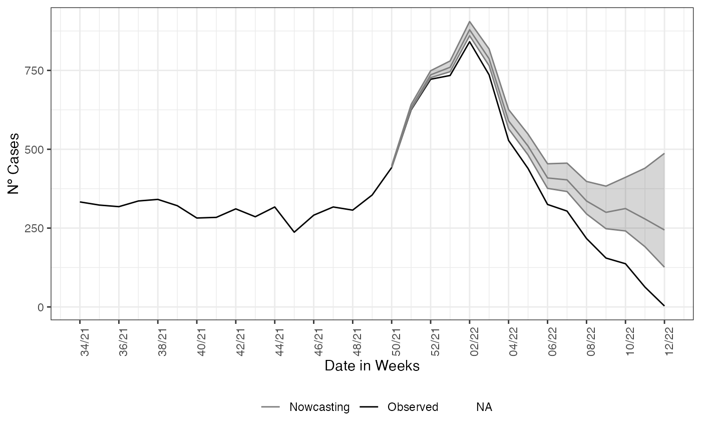
Structured data, Age
The first improvement we have done on the baseline model for nowcasting with a non-structured data is to have the same model for categorical class of the case counts, due to the epidemiological course of SARS-CoV-2, we expect to different ages having different delays distribution. We call this kind of looking into to the data as the structured data, as the data now have identifiers for time, delay and the age class of the cases. To the structured data we fit again a Negative binomial distribution to the cases count at time with delay . Differently, from the non-structured case the model now gives random effects to the delay distribution and time distribution by each of the age-class chosen by the user to break the data. The model has the form now:
$$\begin{equation}Y_{t,d,a} \sim NegBinom(\lambda_{t,d,a}, \phi), \\ \log(\lambda_{t,d,a}) = \alpha_a + \beta_{t,a} + \gamma_{d,a}, \\ \beta_{t,a} := u_t - u_{(t-1)} - u_{(t-2)} \sim N(0,\tau_{a, \beta}); \gamma_{d,a} := u_d - u_{(d-1)} \sim N(0, \tau_{a, \gamma}) \\ t=1,2,\ldots,T, \\ d=1,2,\ldots,D, \\ a=1,2,\ldots,A, \\ \end{equation}$$
where each age class,
,
has an intercept
following a Gaussian distribution with a very large variance, the
time-age random effects,
,
follow a joint multivariate Gaussian distribution with a separable
variance components an independent Gaussian term for the age classes
with precision
and a second order random walk term for the time with precision
.
Analogously, the delay-age random effects,
,
follow a joint multivariate Gaussian distribution with a separable
variance components an independent Gaussian term for the age classes
with precision
and a first order random walk term for the time with precision
.
The model is then completed by INLA default prior distributions for
,
,
,
and
.
See nbinomial,
rw1
and rw2
INLA help pages.
This new model corrects the delay taking into account the effects of
age classes and the interactions of each age class between time and also
delay. Now the model needs a flag indicating which is the column on the
data set which will be used to break the data into age classes and
another parameter flagging on how the age classes will be split. This is
given by the parameters age_col and bins_age.
We also pass two additional parameters, data.by.week to
return the epidemiological curve out of window of action of nowcasting
estimate and return.age to inform we desire a nowcasting
result in two ways, the total aggregation estimate and the
age-stratified estimate. The calling of the function has the following
form:
nowcasting_bh_age <- nowcasting_inla(dataset = sragBH,
                                     bins_age = "10 years",
                                     data.by.week = T,
                                     date_onset = DT_SIN_PRI,
                                     date_report = DT_DIGITA,
                                     age_col = Idade)
Each of the estimates returned by nowcasting_inla has
the same form as in the non-structured case. On the nowcasting
estimates, it returns a data.frame with the posterior
median and 50% and 95% credible intervals, (LIb and LSb) and (LI and LS)
respectively.
library(ggplot2)

dados_by_week <- nowcasting_bh_age$data |>
  dplyr::group_by(dt_event) |>
  dplyr::reframe(
    observed = sum(Y, na.rm = T)
  ) |>
  dplyr::filter(dt_event >= max(dt_event)-270)


nowcasting_bh_age$total |>
  ggplot()+
  geom_line(aes(x = dt_event, y = Median,
                col = 'Nowcasting'))+
  geom_line(data = dados_by_week,
            aes(x = dt_event, y = observed,
                col = "Observed"))+
  geom_ribbon(aes(x = dt_event, y = Median,
                  ymin = LI, ymax = LS),
              alpha = 0.2, show.legend = F)+
  theme_bw()+
  theme(legend.position = "bottom", axis.text.x = element_text(angle = 90))+
  scale_color_manual(values = c('grey50', 'black'), name = '')+
  scale_x_date(date_breaks = '2 weeks', date_labels = '%V/%y', name = 'Date in Weeks')+
  labs(x = '', y = 'Nº Cases')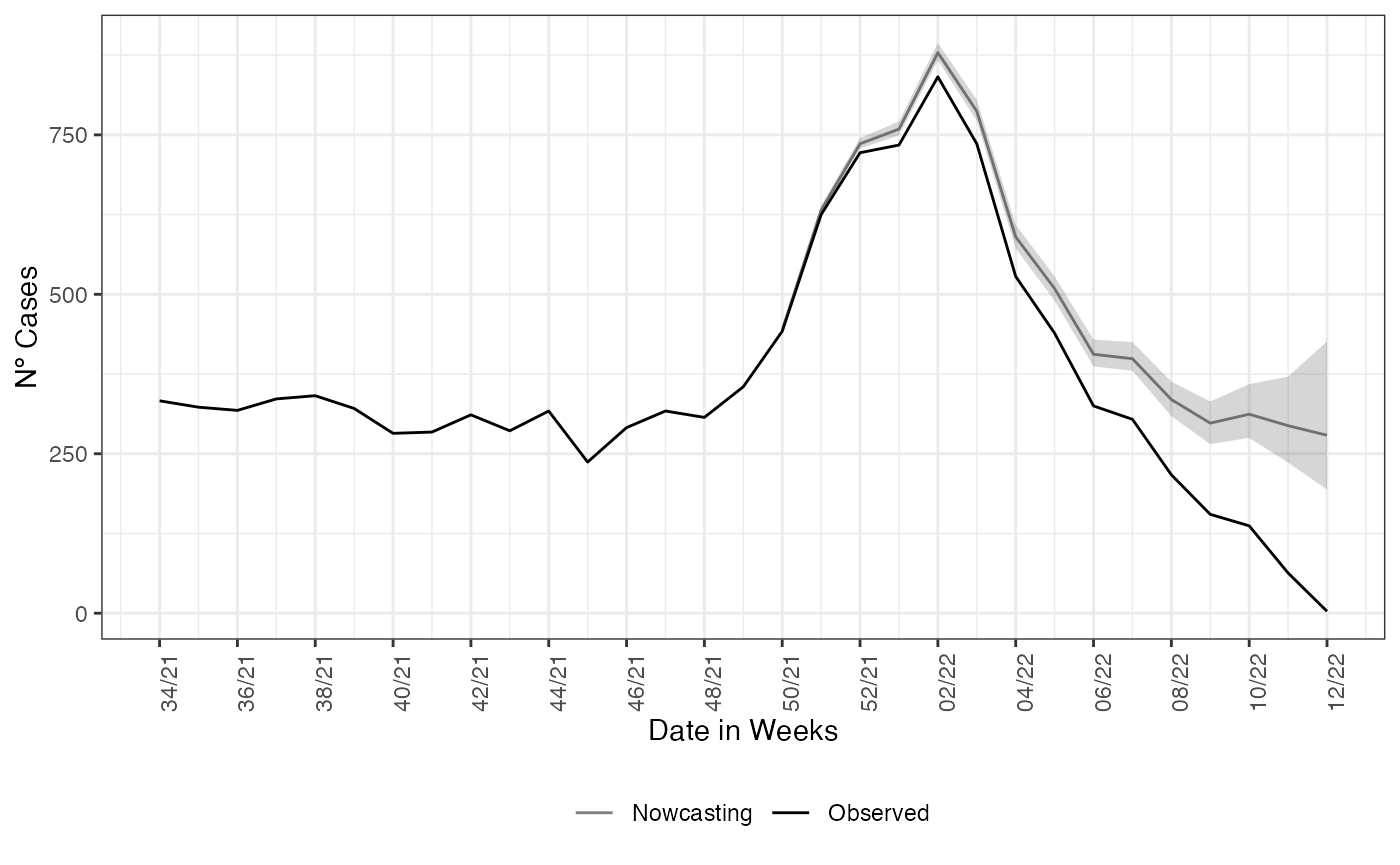
For sake of completeness we plot both estimates together to check how different they are.
ggplot()+
  geom_line(data = dados_by_week,
            aes(x = dt_event, y = observed,
                color = "Observed"))+
  geom_line(data = nowcasting_bh_no_age$total |>
              filter(dt_event >= (max(dt_event)-270)),
            aes(x = dt_event, y = Median,
                color = 'Nowcasting - Non-structured'))+
  geom_ribbon(data = nowcasting_bh_no_age$total |>
              filter(dt_event >= (max(dt_event)-270)),
              aes(x = dt_event, y = Median,
                  ymin = LI, ymax = LS,
                  fill = "Nowcasting - Non-structured"),
              alpha = 0.5, show.legend = F)+
  geom_line(data = nowcasting_bh_age$total |>
              filter(dt_event >= (max(dt_event)-270)),
            aes(x = dt_event, y = Median,
                color = 'Nowcasting - Structured'))+
  geom_ribbon(data = nowcasting_bh_age$total |>
              filter(dt_event >= (max(dt_event)-270)),
              aes(x = dt_event, y = Median,
                  ymin = LI, ymax = LS,
                  fill = "Nowcasting - Structured"),
              alpha = 0.5, show.legend = F)+
  theme_bw()+
  theme(legend.position = "bottom",
        axis.text.x = element_text(angle = 90))+
  scale_color_manual(values = c("lightblue4",
                                "orange4",
                                "black"),
                     name = "")+
  scale_fill_manual(values = c("lightblue1",
                                "orange1",
                                "black"),
                    name = "")+
  scale_x_date(date_breaks = '2 weeks',
               date_labels = '%V/%y',
               name = 'Date in Weeks')+
  labs(x = '',
       y = 'Nº Cases')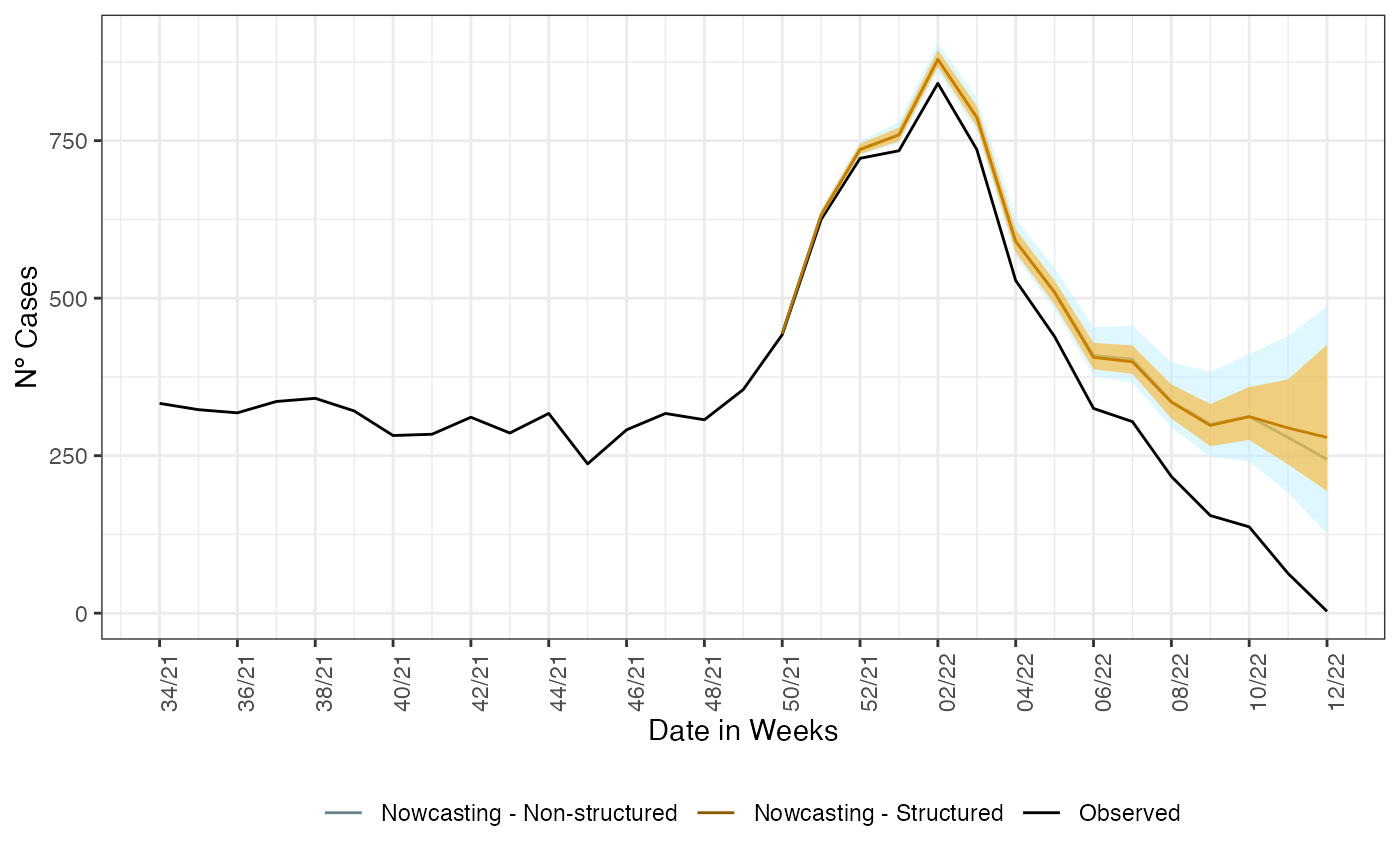
The nowcasting when using the age information is narrower and shows a less decreasing tendency at the end of the time series. This is due to as each age classes have a nowcasting model acting on it, it can capture effects once mascaraed when not breaking it by age.
Conclusion
Over this vignette we learned how to use the
nowcasting_inla() and how nowcaster can employ
two different models, one without considering differences of delay by
age class and another considering differences of delay per age classes.
Finally, we compared both estimates, showing that the model that uses
the age class information to nowcasting produce narrower estimates