First example on LazyData
When the package is loaded it provides a Lazy Data file,
sariBH, it is a anonymized records of Severe Acute
Respiratory Illness notified in the city of Belo Horizonte, since March
2020 to April 2022. To load it basically write:
library(INLA)
library(parallel)
library(nowcaster)
# Loading Belo Horizonte SARI data set
data(sragBH)
And we take a look on the data:
head(sragBH)
#>   DT_SIN_PRI  DT_DIGITA CLASSI_FIN EVOLUCAO CO_MUN_RES Idade fx_etaria
#> 1 2020-02-11 2020-03-05          4        1     310620    59   50 - 59
#> 2 2020-01-21 2020-02-06          4        1     310620    79   70 - 79
#> 3 2020-03-30 2020-04-17          4        1     310620    72   70 - 79
#> 4 2020-03-26 2020-04-02          4        1     310620    82      80 +
#> 5 2020-03-20 2020-04-13          4        1     310620    50   50 - 59
#> 6 2020-04-07 2020-04-22          5        1     310620    74   70 - 79
It is a data.frame with 7 variables and 65,404 observations. We will make use of only the first two columns, “DT_SIN_PRI” (date of onset symptoms) and “DT_DIGITA” (recording date) as well the column “Idade” (age in years) to make age structured nowcasting.
The call of the function is straightforward, it simply needs a data
set as input, here the LazyData loaded in the namespace of
the package. The function has 3 mandatory parameters,
dataset for the parsing of the data set to be nowcasted,
date_onset for parsing the column name which is the date of
onset of symptoms and date_report which parses the column
name for the date of report of the cases. Here this columns are
“DT_SIN_PRI” and “DT_DIGITA”, respectively.
nowcasting_bh_no_age <- nowcasting_inla(dataset = sragBH,
                                        date_onset = "DT_SIN_PRI",
                                        date_report = "DT_DIGITA",
                                        data.by.week = T)
head(nowcasting_bh_no_age$total)
#> # A tibble: 6 × 7
#>    Time dt_event   Median    LI    LS   LIb   LSb
#>   <int> <date>      <dbl> <dbl> <dbl> <dbl> <dbl>
#> 1    17 2021-12-13    444  442    448   443  445
#> 2    18 2021-12-20    632  626    641   629  634
#> 3    19 2021-12-27    736  728    750   733  741
#> 4    20 2022-01-03    759  747.   780   754  765.
#> 5    21 2022-01-10    878  862    903   871  886
#> 6    22 2022-01-17    787  765    816   778  795
This calling will return for the first element the nowcasting
estimate and its Credible Interval (CI) for two different credibility
levels, LIb and LSb are the CI limits for 50%
of credibility, and LI and LS are CI limits
for a 95% credibility.
On the second element it returns the data to be grouped and summarized to give the epidemic curve, we can take a look on this element.
library(ggplot2)
library(dplyr)

dados_by_week <- nowcasting_bh_no_age$data |>
  dplyr::group_by(dt_event) |>
  dplyr::reframe(
    observed = sum(Y, na.rm = T)
  ) |>
  dplyr::filter(dt_event >= max(dt_event)-270)

dados_by_week |>
  ggplot()+
  geom_line(data = dados_by_week,
            aes(dt_event,
                y = observed,
                col = 'Observed'))+
  theme_bw()+
  theme(legend.position = "bottom",
        axis.text.x = element_text(angle = 90)) +
  scale_color_manual(values = c('grey50', 'black'),
                     name = '')+
  scale_x_date(date_breaks = '2 weeks',
               date_labels = '%V/%y',
               name = 'Date in Weeks')+
  labs(x = '',
       y = 'Nº Cases')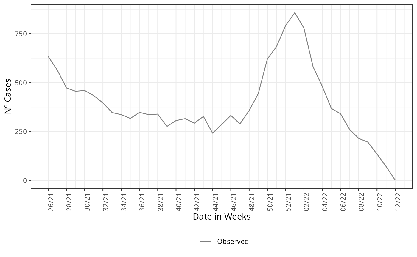
After this element is grouped by and summarized by the onset of
symptoms date, here DT_SIN_PRI, it is the epidemiological
curve observed. To example how the estimate compares with the observed
curve, we plot the estimate and the epidemiological curve all
together.
nowcasting_bh_no_age$total |>
  ggplot(aes(x = dt_event, y = Median,
             col = 'Nowcasting')) +
  geom_line(data = dados_by_week,
            aes(y = observed,
                col = 'Observed'))+
  geom_ribbon(aes(ymin = LI, ymax = LS), col = NA,
              alpha = 0.2,
              show.legend = F)+
  geom_line()+
  theme_bw()+
  theme(legend.position = "bottom",
        axis.text.x = element_text(angle = 90)) +
  scale_color_manual(values = c('grey50', 'black'),
                     name = '')+
  scale_x_date(date_breaks = '2 weeks',
               date_labels = '%V/%y',
               name = 'Date in Weeks')+
  labs(x = '',
       y = 'Nº Cases')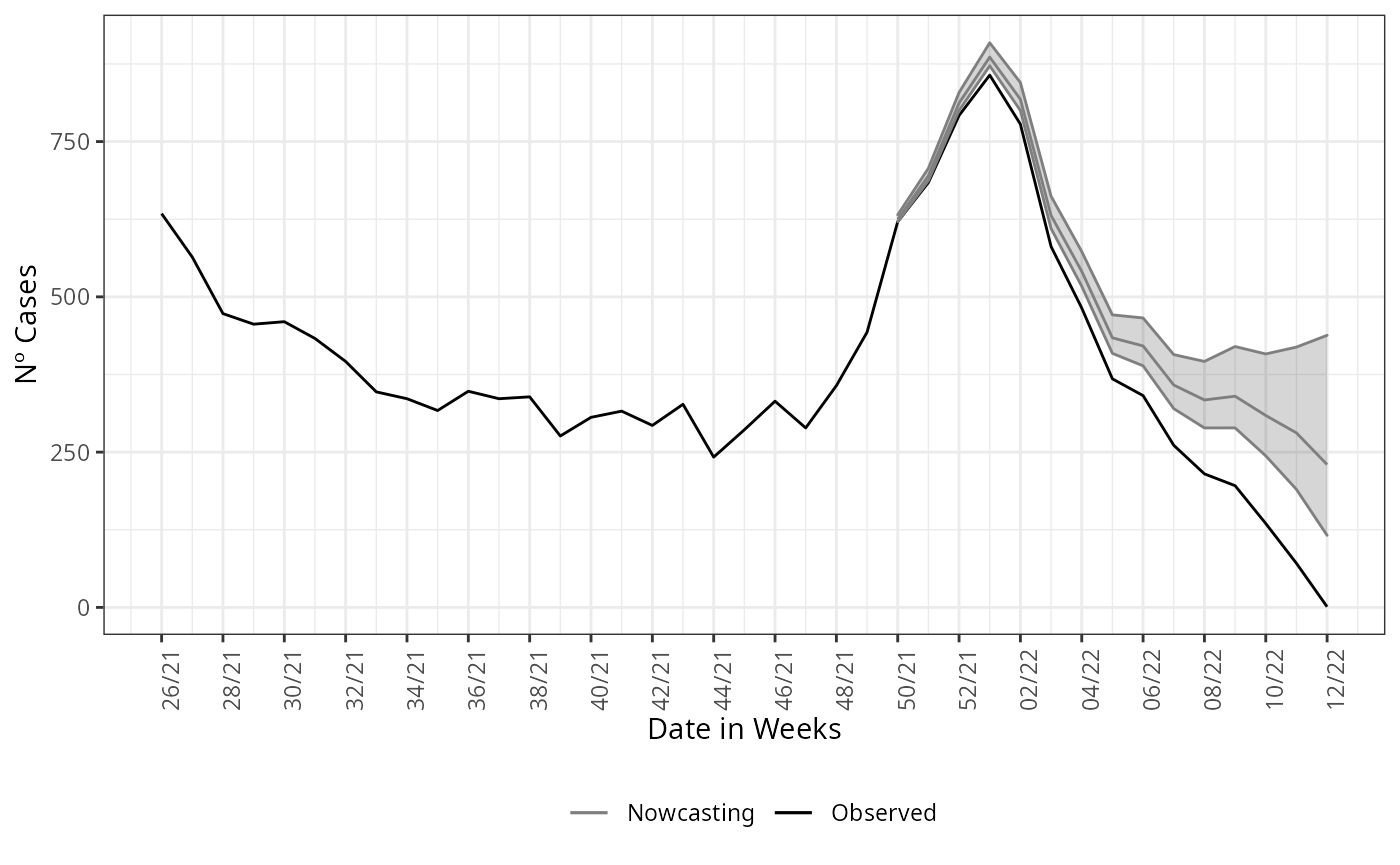
This is an example were the estimate was done without considering any type of structure in data, which is the first assumption for the nowcasting.